Development of an Image Generation module via Diffusion Models

May 1, 2025 • 21 min read (+28 min annexes) • By Héctor Tablero Díaz , Álvaro Martínez Gamo

Exploring, implementing and comparing different Diffusion Models for image generation.

WARNING

This page was translated with AI. The content may not be accurate.

Abstract

This work presents the development of a Python software package for image generation via diffusion models. Diffusion models represent an emerging class of generative models that have demonstrated exceptional results in creating high-quality images, surpassing in many aspects previous techniques like Generative Adversarial Networks (GANs).

Our package implements three main variants of diffusion processes: Variance Exploding (VE), Variance Preserving (VP), and Sub-Variance Preserving (Sub-VP), each with distinctive characteristics for different use cases. For the sampling process, we provide four implementations: Euler-Maruyama, Predictor-Corrector, Probability Flow ODE, and Exponential Integrator, allowing for a balance between speed and quality according to specific requirements. Complementarily, we include two noise schedulers (linear and cosine) that control the addition of noise during the diffusion process.

A notable feature of the package is its capacity for controllable generation, including grayscale image colorization, imputation of missing regions, and class-conditioned generation. These functionalities significantly expand the scope of practical applications, from image restoration to the creation of specific content.

To ensure usability, we designed an intuitive programming interface complemented by an interactive dashboard, facilitating both programmatic use and visual experimentation. The package also includes standard metrics (BPD, FID, IS) for the quantitative evaluation of results.

The experiments performed demonstrate the effectiveness of our implementation in various generative tasks, producing high-quality images even with models trained on limited datasets. The code is structured in a modular and extensible way, facilitating the incorporation of new functionalities and adaptation to specific use cases.

The system includes innovative tools for secure serialization, an interactive dashboard, and auto-generated documentation, exceeding basic requirements.

1. Introduction

Image generation via machine learning represents one of the most fascinating and rapidly developing fields within artificial intelligence. In recent years, we have witnessed significant advances that have transformed our ability to create high-quality visual content automatically.

In this context, diffusion models have emerged as a particularly promising paradigm, offering substantial advantages over previous approaches like Generative Adversarial Networks (GANs). Their theoretical foundation in well-established stochastic processes provides an elegant framework for image generation, with more stable training and high-fidelity results.

This project focuses on the development of a Python software package for diffusion-based image generation, which implements different variants of these processes and provides flexibility regarding sampling methods, noise scheduling, and controllable generation tasks. Our implementation allows not only for generating images from random noise but also for more specific tasks like colorizing grayscale images, imputing missing regions, and class-conditioned generation.

The package has been designed with an emphasis on modularity and extensibility, allowing users to adapt each component according to their specific needs. Furthermore, it includes commonly used evaluation metrics in the field to facilitate comparison between different configurations and with other generation methods.

Motivation

The main motivation for developing this package stems from the need for accessible and flexible tools for the research and application of diffusion models. While there are reference implementations for specific models, we consider it valuable to provide a library that allows for experimenting with different configurations and systematically comparing their performance.

Moreover, the incorporation of controllable generation capabilities responds to the growing demand for methods that allow for greater control over the generative process, facilitating its application in contexts where certain constraints or specific characteristics in the generated images must be respected.

Another key motivation is facilitating research with custom components, simplifying the process of sharing models between teams. Our system serializes both trained parameters and the necessary class definitions, eliminating the need to manually share source code or maintain exact dependencies between environments. To ensure security, we implement an optional loading mechanism that requires explicit user confirmation and executes the code in a restricted environment, thus allowing collaboration without compromising system security.

Objectives

The main objectives of this project are:

Develop a modular and extensible library for image generation via diffusion models.
Implement different variants of diffusion processes, sampling methods, and noise schedules.
Incorporate functionalities for controllable generation, including colorization, imputation, and class conditioning.
Provide standard metrics for evaluating the quality of generated images.
Create an interactive user interface to facilitate experimentation with the different components of the package.
Thoroughly document both the code and the underlying theoretical foundations.
Implement a secure serialization system for loading and saving custom classes.

Document Structure

The remainder of this document is organized as follows:

Chapter Development presents the software development, including work planning, requirements analysis, package design, and testing performed.

Chapter Results describes the results obtained, including examples of package usage and the project conclusions.

Finally, several appendices are included with additional technical material, complementary examples, and exhaustive comparisons between different package configurations.

1.1. State of the Art

The field of image generation via machine learning techniques has advanced significantly in recent years, with diffusion models standing out. These models have proven to be a promising alternative to Generative Adversarial Networks (GANs) and autoregressive models, offering high-quality samples with more stable training.

Diffusion Models

Diffusion models are based on a process that gradually adds noise to data and then learns to reverse this process. This approach provides a theoretically grounded framework in Stochastic Differential Equations (SDEs), where the process of adding noise defines a trajectory from the original data to pure noise, and the reverse process allows for generating new samples.

Among the most notable implementations is Stable Diffusion, which operates in a compressed latent space rather than the full pixel space, significantly reducing computational requirements. This approach allows for generating high-resolution images while maintaining training stability, using a Variational Autoencoder (VAE) to compress and decompress the representation before and after the diffusion process.

Colorization without Retraining

A notable advance in the field is CGDiff (Color-Guided Diffusion), a method that allows for colorizing grayscale images without the need to retrain the model. This technique is based on manipulating the latent space of the diffusion model, guiding the generation process to preserve the structural information of the original image while adding plausible chromatic information.

The CGDiff approach is particularly interesting because it demonstrates the flexibility of diffusion models for conditional generation tasks, leveraging the knowledge already acquired by the model about the distribution of natural images.

Trends in Image Imputation

Image imputation, also known as inpainting, seeks to complete missing regions coherently with the surrounding content. The most recent diffusion-based techniques have surpassed previous methods thanks to their ability to generate more coherent and detailed completions.

The current state of research focuses on guided sampling techniques, where additional information is used to condition the generation process, allowing for precise control over the generated content. These techniques allow for preserving specific details while completing missing regions, maintaining the global coherence of the image.

Text-to-Image Generation

Although not the main focus of our project, we cannot fail to mention advances in text-to-image models like DALL-E 2 and Imagen, which have demonstrated the capability of diffusion models to generate detailed images from textual descriptions. These models incorporate text representations learned by models like CLIP or T5, which allow aligning the semantic space of text with the visual space of images.

The relevance of these advances for our work lies in the conditioning techniques they employ, which in many cases are generalizable to other types of conditioning, such as class-based generation implemented in our project.

2. Development

This chapter details the development process of the software package for image generation via diffusion models. It addresses the different phases of development, from initial planning to validation and testing, including requirements analysis and system architecture design.

Development has been carried out following an iterative and incremental approach, prioritizing code modularity and extensibility. This has allowed for progressively implementing the different functionalities and system components, facilitating continuous integration and unit testing.

The methodology employed has placed special emphasis on code quality, thorough documentation, and ease of use, both for end users and for developers wishing to extend or modify the system. Throughout the process, version control tools, automated testing, and integrated documentation have been used to ensure software robustness and maintainability.

The following sections describe in detail each aspect of the development, from planning to validation, including considerations about software quality assurance and other relevant issues.

2.1. Work Planning

To carry out the work, we planned and divided the tasks equitably with the support of a Gantt chart to approximately follow the deadlines, taking into account that for logistical reasons we have less time than scheduled to complete it.

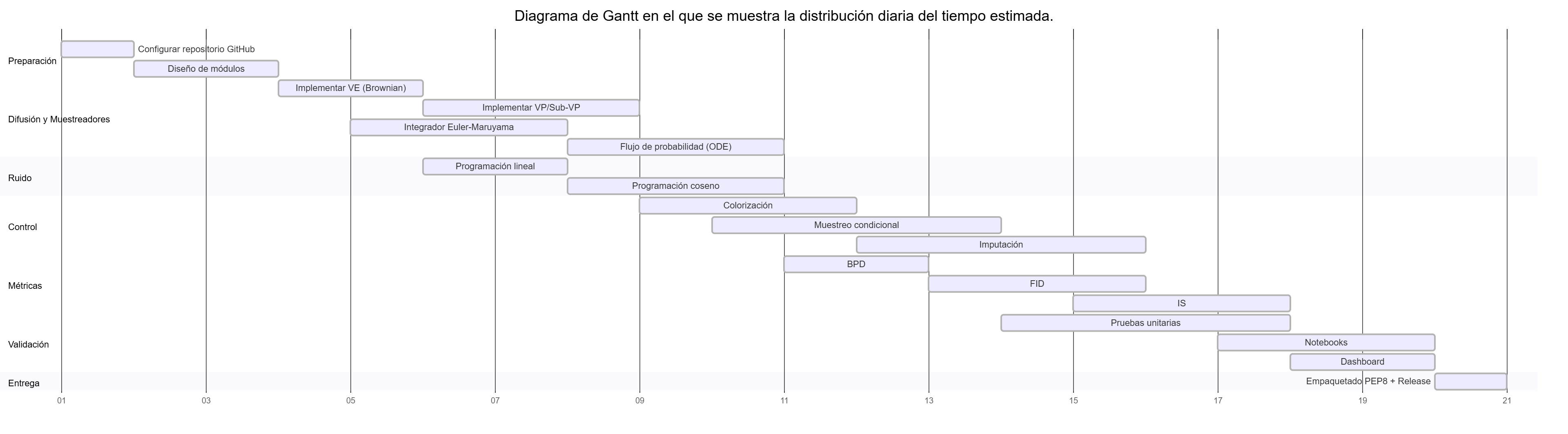
Gantt chart showing the estimated daily time distribution.

Although this was our original idea, we ultimately could not meet the established deadlines, and it was necessary to use the 50 days granted for the project’s completion. While most classes were finished according to the diagram, the extra work, as well as adjusting default parameters and bug fixes, took much longer than expected.

2.2. Requirements Analysis

2.2.1. Functional Requirements

The software must provide the following functionalities:

RF-1. Allow image generation via diffusion models.
- RF-1.1. Support generating images from random noise.
- RF-1.2. Facilitate imputation of missing regions in partial images.
- RF-1.3. Include the option for generation conditioned to a specific class.
RF-2. Offer configurations to control the parameters of the generative process.
RF-3. Support different sampling methods for image generation.
RF-4. Include metrics to evaluate the quality of generated images.
RF-5. Provide an easy-to-use interface via a Python API.
RF-6. Allow integration with Jupyter notebooks for demonstrations and testing.

2.2.2. Non-Functional Requirements

These are the constraints to which the software is subject:

RNF-1. The generation time for a $32 \times 32$ $32 \times 32$ pixel image must not exceed:
- RNF-1.1. 5 seconds when running on a GPU with CUDA.
- RNF-1.2. 10 seconds when running on a CPU with at least 4 cores.
RNF-2. The maximum RAM consumption must not exceed 8 GB during standard model execution.
RNF-3. The code must follow Google’s style guides to ensure clarity and maintainability.
RNF-4. The documentation must include usage examples to facilitate software adoption.
RNF-5. The system must be compatible with Python 3.9 or higher and use standard machine learning libraries, including PyTorch $\geq$ 2.0.0.

2.2.3. Use Cases

The use cases describe how a user would interact with the system:

CU-1. Generation of images from random noise: The user configures parameters such as size and sampling method. The system generates the image and returns it in a compatible format (png, jpg).
CU-2. Imputation of missing regions in partial images: The user provides an image with missing areas. The system completes them based on the surrounding content and returns the reconstructed image.
CU-3. Generation of images conditioned to a class: The user selects a category (e.g., “dog” or “cat”). The system generates the corresponding image and returns it in a compatible format.

2.3. Design

The design of the Python module has been done with a focus on extensibility and modularity, following object-oriented design principles and interface programming. The system architecture is based on abstract classes that define interfaces, along with concrete implementations that provide specific behaviors.

This structure facilitates both basic package usage for users with standard needs, and extension and customization for advanced users requiring specific behaviors. An example of this approach can be seen in the ‘samplers.ipynb’ notebook, which demonstrates how to use and combine different sampler implementations.

Design Patterns

Several design patterns have been applied to improve the structure and flexibility of the code:

Strategy Pattern: Used in the different diffusers, samplers, and noise schedulers, allowing components to be easily swapped.
Factory Pattern: Implemented in the GenerativeModel class to create instances of the different components based on configuration parameters.
Observer Pattern: Used for tracking progress during image generation.

Modular Architecture

The system architecture has been designed to maximize cohesion within each module and minimize coupling between modules. Each component has a clear and well-defined responsibility:

Diffusion Module: Encapsulates the algorithms that define how noise is added and removed during the diffusion process.
Sampling Module: Implements different strategies for numerically solving the stochastic differential equations of the diffusion process.
Noise Scheduling Module: Defines how noise is distributed throughout the diffusion process.
Metrics Module: Provides tools for evaluating the quality of generated images.

User Interface

The package provides two main interfaces:

Programmatic API: A Python interface that allows access to all package functionalities through code.
Interactive Dashboard: A Streamlit-based graphical interface that facilitates experimentation and demonstration of system capabilities without the need to write code. In addition to the local version, an online version (without GPU) can be accessed via https://image-gen-htd.streamlit.app/.

The dashboard represents a significant contribution to the system’s usability, allowing users with different levels of technical experience to interact with diffusion models in an intuitive way.

Extension System

A distinctive feature of the design is the dynamic loading system for custom classes, which allows users to extend system behavior without modifying the base code. This functionality is implemented through the CustomClassWrapper class, which provides secure mechanisms for loading and executing user-defined code.

This class is managed internally by the system, and users can load models with custom classes as if they were loading a normal one, improving the user experience and allowing for greater flexibility in system customization.

2.3.1. Package Structure

Regarding the file structure, the module code has been distributed into subfolders as follows:

diffusion/
    |-- base.py
    |-- ve.py
    |-- vp.py
    |-- sub_vp.py
metrics/
    |-- base.py
    |-- bpd.py
    |-- fid.py
    |-- inception.py
noise/
    |-- base.py
    |-- linear.py
    |-- cosine.py
samplers/
    |-- base.py
    |-- euler_maruyama.py
    |-- exponential.py
    |-- ode.py
    |-- predictor_corrector.py
base.py
score_model.py
visualization.py
utils.py

Additionally, the project includes code for generating an interactive dashboard, tests, documentation, and an additional folder containing example notebooks. The complete code structure would be as follows:

dashboard/
    |-- (styles and languages)
.streamlit/
    |-- config.toml
dashboard.py
examples/
    |-- class_conditioning.ipynb
    |-- colorization.ipynb
    |-- diffusers.ipynb
    |-- evaluation.ipynb
    |-- getting_started.ipynb
    |-- imputation.ipynb
    |-- noise_schedulers.ipynb
    |-- samplers.ipynb
docs/
    |-- (markdown with documentation)
tests/
    |-- (various tests)

2.3.2. Class Diagram

Our package’s architecture is designed following object-oriented programming and modular design principles. The class diagram presented in Figure Class diagram of the image generation package shows the relationships between the main components of the system.

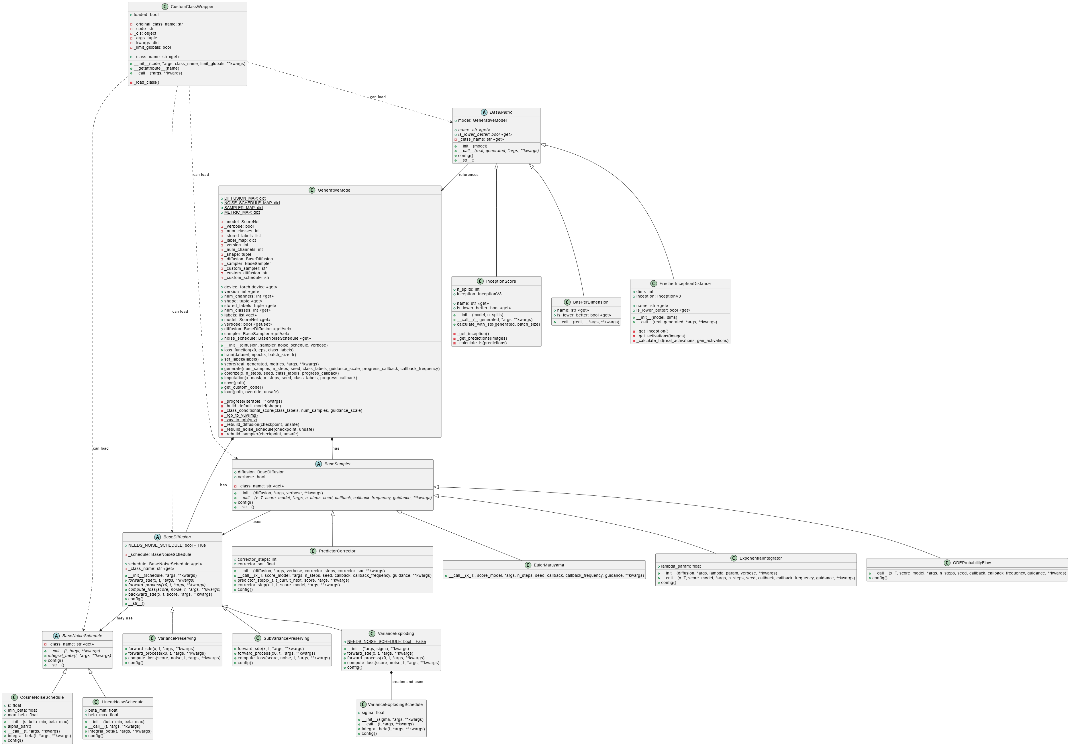
Class diagram of the image generation package.

The diagram illustrates the hierarchical structure of the classes and their interactions:

The GenerativeModel class acts as the central point, coordinating the diffusion, sampling, and noise scheduling components.
Each category of components (diffusers, samplers, and noise schedulers) follows a design pattern with abstract base classes that define common interfaces.
Concrete implementations inherit from these base classes and provide specific behaviors.
The metrics system follows a similar design, with a base class BaseMetric and specializations for each specific metric.

This design allows for system extensibility, facilitating the addition of new implementations without modifying existing code. For example, a user can create a new type of diffuser by inheriting from BaseDiffusion and implementing the required abstract methods.

The design’s flexibility is also reflected in how the different components can be combined. For example, any diffuser can be used with any sampler, as long as both correctly implement their respective interfaces.

2.4. Validation and Testing

The validation and testing process has been an essential component in the development of our software package, ensuring that all functionalities meet the established requirements and provide correct and consistent results.

Testing Strategy

Unit Tests: Verify the correct behavior of isolated individual components.
Integration Tests: Validate the correct interaction between different modules.
System Tests: Check the functioning of the complete system in real usage scenarios.
Performance Tests: Evaluate execution times and resource consumption.

Unit Tests

Unit tests have been implemented using the pytest framework, with a fixture-based approach to facilitate the setup of test scenarios. Specific tests have been developed for each system module:

test_diffusion.py: Verifies the behavior of the different diffusion processes.
test_samplers.py: Checks the functioning of the sampling methods.
test_noise.py: Validates the noise schedulers.
test_metrics.py: Ensures the correct implementation of evaluation metrics.
test_base.py: Tests the functionality of the GenerativeModel class.

Unit tests cover both typical cases and edge and error scenarios, ensuring that all components properly handle exceptional situations.

Integration Tests

Integration tests, implemented in test_integration.py, verify the correct interaction between the different system modules. These tests simulate complete workflows, including:

Model training and image generation.
Image colorization and imputation.
Class-conditioned generation.
Model saving and loading.

Performance Tests

Performance tests have been conducted to evaluate:

Generation times for different configurations (see Figure Generation times per configuration and sampler).
Memory consumption during training and generation.
Scalability with the number of steps.

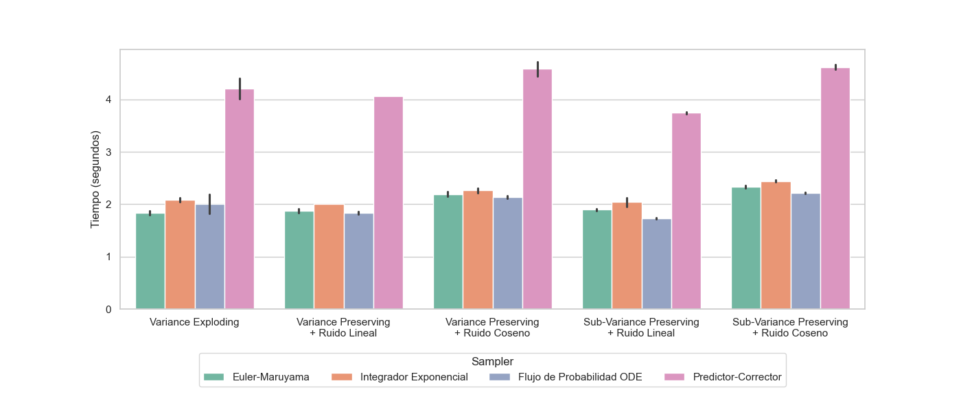
Generation times per configuration and sampler (MNIST, partial dataset, unconditional generation).

Exhaustive comparisons can be found in the appendix Exhaustive Comparisons.

Compatibility and Environments

The package’s compatibility with various hardware configurations has been verified:

Systems with CUDA GPU.
Systems with CPU only.
Different operating systems (Windows and Linux).

2.5. Software Quality Assurance

Quality assurance has been a fundamental aspect in the development of our software package. We have implemented various practices and tools to ensure that the code is robust, maintainable, and compliant with industry standards.

Version Control

Development has been carried out using Git as a version control system, with a repository hosted on GitHub. This has facilitated:

Detailed tracking of code changes.
Coordinated collaborative development.
Code review via pull requests.

The package source code can be found at the following link: https://github.com/HectorTablero/image-gen.

Coding Standards

The code has been developed following Google’s style guides for Python, ensuring consistency and readability.

Documentation

Documentation has been a priority throughout development, implemented at several levels:

API Documentation: Automatically generated from docstrings in Google format.
User Documentation: Includes manuals, tutorials, and usage examples.
Example Notebooks: Demonstrate specific use cases with executable examples.
Code Comments: Explain complex or non-intuitive sections.

Documentation is automatically generated using MkDocs and published via GitHub Pages, ensuring it is always up to date with the latest code version. It can be consulted here: https://hectortablero.github.io/image-gen/.

Additionally, a version of the documentation generated by Devin can be found at the following link: https://deepwiki.com/HectorTablero/image-gen.

Dependency Management

Project dependencies are managed via:

requirements.txt and pyproject.toml files that specify dependencies and their versions.
Virtual environments to isolate development and avoid conflicts.

2.6. Other Considerations

The software developed in this project is distributed under the MIT license, which allows its use, modification, and redistribution without significant restrictions, provided the original attribution is maintained. However, no warranties of any kind are provided, and the developers assume no liability for its use.

The user is solely responsible for the use of the software and must ensure compliance with applicable laws in their jurisdiction. In particular, the use of the software to generate inappropriate, misleading, or third-party rights infringing content is strictly discouraged.

3. Results

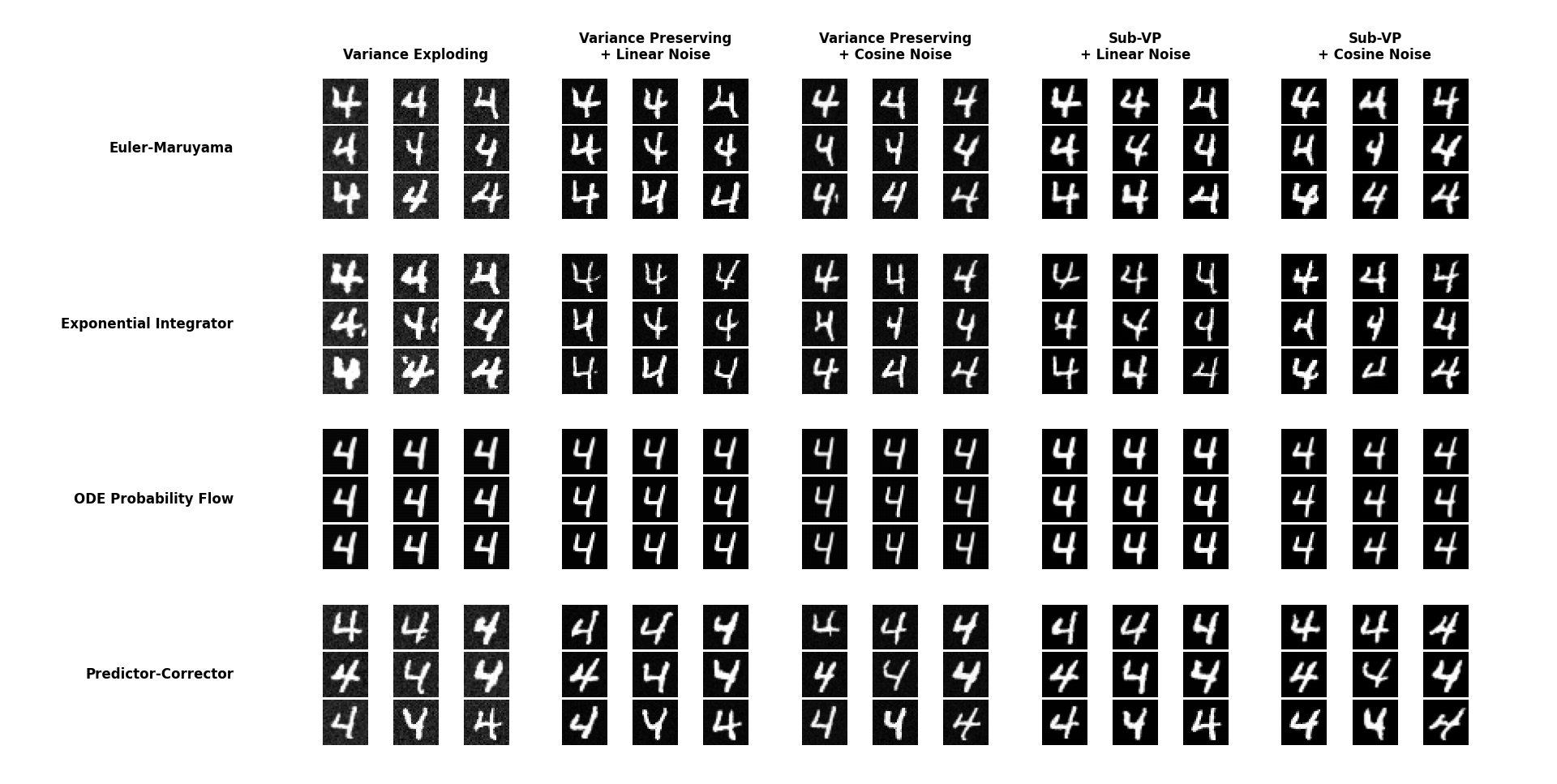
Below are results from image generation of models trained with images of ships from the CIFAR-10 dataset (Figure Generated images training with CIFAR-10, 100 epochs) and with images of fours from MNIST (Figure Generated images training with MNIST, 100 epochs):

Generated images training with CIFAR-10, 100 epochs.

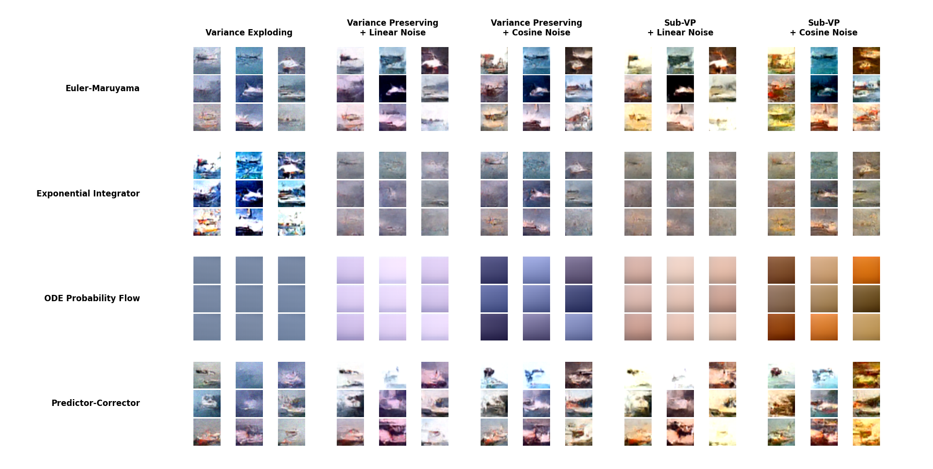
Sub-Variance Preserving is the diffuser that takes the longest to learn the data distribution. In this case, the model trained with only 100 epochs, so it hasn’t had enough time to learn to distinguish well between ships and the rest of the dataset.
ODE is deterministic and converges to the mean of the learned data distribution, so it may not generate satisfactory results in some cases. In the case of MNIST, the generation is considerably better:

Generated images training with MNIST, 100 epochs.

3.1. Usage Examples

In this section, we present various usage examples of our package that illustrate its capabilities and functionalities. These examples are available as Jupyter notebooks in the project repository, allowing users to reproduce them and experiment with different configurations.

Basic Image Generation

The following code shows how to initialize a generative model with default configuration and generate a set of images:

from image_gen.visualization import display_images
from image_gen import GenerativeModel

# Initialize model with Variance Exploding diffusion and Euler-Maruyama sampler
model = GenerativeModel(diffusion="ve", sampler="euler-maruyama")
model.train(dataset, epochs=25)

# Generate 4 images with 500 sampling steps
images = model.generate(num_samples=4, n_steps=500, seed=42)

# Visualize the generated images

Figure: Basic Generation

Image Colorization

The following example shows how to use the model to colorize a grayscale image:

# Load a pre-trained model
model = GenerativeModel.load("saved_models/cifar10.pth")

# Create a grayscale image (averaging RGB channels)
color_image = model.generate(num_samples=1)[0]
gray_image = torch.mean(color_image, dim=0, keepdim=True).unsqueeze(0)

# Colorize the image
colorized = model.colorize(gray_image, n_steps=500)

# Visualize original in grayscale and colorized version
display_images(gray_image)
display_images(colorized)

Figure: Image Colorization

Region Imputation

This example shows how to perform imputation of missing regions in an image:

# Load model
model = GenerativeModel.load("saved_models/cifar10.pth")

# Generate base image
base_image = model.generate(num_samples=1)

# Create mask (1 = region to generate, 0 = preserve)
mask = torch.zeros_like(base_image)
h, w = base_image.shape[2], base_image.shape[3]
mask[:, :, h//4:3*h//4, w//4:3*w//4] = 1  # Central rectangular mask

# Perform imputation
results = model.imputation(base_image, mask, n_steps=500)

# Visualize result
display_images(torch.cat([base_image, results], dim=0))

Figure: Image Imputation

Additional examples can be consulted in the appendix Additional Examples, where more advanced use cases are presented.

3.2. Conclusions

The development of this diffusion model-based image generation package has allowed for the implementation and evaluation of different variants of these models, demonstrating their effectiveness in various generation tasks, from creating images from random noise to more specific tasks like colorization and imputation.

Achievements and Contributions

The main achievements and contributions of this project are:

Implementation of three variants of diffusion processes (VE, VP, and Sub-VP), allowing for comparison of their performance in different scenarios.
Development of four sampling methods with different quality and efficiency characteristics, providing flexibility for different use cases.
Incorporation of controllable generation capabilities that significantly expand the package’s utility.
Creation of a modular and extensible architecture that facilitates the incorporation of new components.
Development of an interactive dashboard that significantly improves the package’s accessibility.
Implementation of standard metrics for the quantitative evaluation of generated image quality.

Experimental results confirm that diffusion models represent a viable alternative to other generative techniques, with the additional advantage of more stable training and a solid theoretical framework based on stochastic differential equations.

Limitations

Despite the positive results, it is also important to recognize the current limitations of the package:

Generation time remains considerably higher than other generative techniques like GANs, especially when more sophisticated sampling methods are used.
The quality of generated images, although good, still does not reach the level of more specialized implementations like Stable Diffusion, which operate in compressed latent spaces.
Training models for high-resolution images requires significant computational resources that have not been fully explored in this project.

Future Work

Based on the results obtained and the limitations identified, several lines of future work could improve and extend this package:

Implementation of latent space diffusion, following the Stable Diffusion approach, to allow efficient generation of higher-resolution images.
Incorporation of sampling acceleration techniques, such as DDIM and DPM-Solver, which could significantly reduce generation time.
Extension to multimodal generation, particularly text-to-image generation.
Development of semantic editing capabilities, allowing modification of specific attributes of generated images.
Optimization of computational performance, especially for use on hardware with limited resources.

Final Considerations

This project demonstrates the potential of diffusion models as a versatile tool for various image generation tasks. The developed modular architecture provides a solid foundation for future developments and extensions, both in academic and practical applications.

We believe that the combination of a well-structured object-oriented design, thorough documentation, and interactive tools like the dashboard significantly contributes to the package’s accessibility and utility, facilitating its adoption by researchers and developers interested in image generation via diffusion models.

In conclusion, this project has not only fulfilled the initial objectives of implementing different variants of diffusion models and evaluating their performance but has also generated a useful and extensible software package that can serve as a foundation for future research and applications.

Appendices

In this appendix, we present additional technical material that delves into the mathematical and algorithmic foundations of the diffusion models implemented in our package.

Stochastic Differential Equations in Diffusion Models

Diffusion models are based on stochastic processes defined by Stochastic Differential Equations (SDEs). For a diffusion process, we define a forward SDE that describes how noise is added to the data, and a backward SDE that governs the noise removal process for generation.

Forward SDE

The forward stochastic differential equation has the general form:

\begin{align} dx = f(x, t)dt + g(t)dw \end{align}

where $f(x, t)$ is the drift term, $g(t)$ is the diffusion coefficient, and $dw$ represents a standard Wiener process.

For the three types of diffusion processes implemented, these terms are specifically defined as:

Variance Exploding (VE):

\begin{align} f(x, t) &= 0 \\\ g(t) &= \sigma^t \end{align}

Variance Preserving (VP):

\begin{align} f(x, t) &= -\frac{\beta(t)}{2}x \\\ g(t) &= \sqrt{\beta(t)} \end{align}

Sub-Variance Preserving (Sub-VP):

\begin{align} f(x, t) &= -\frac{\beta(t)}{2}x \\\ g(t) &= \sqrt{\beta(t) \cdot (1 - e^{-2\int_0^t \beta(s)ds})} \end{align}

Backward SDE

The backward SDE, used for generation, is derived from the forward one and has the form:

\begin{align} dx = [f(x, t) - g(t)^2 \nabla_x \log p_t(x)] dt + g(t) d\bar{w} \end{align}

where $\nabla_x \log p_t(x)$ is the score function (gradient of the logarithm of the density) that is approximated by a neural network during training.

Derivation Demonstration of the Backward SDE

To derive the backward SDE from the forward one, we start with the Fokker-Planck equation, which describes how the probability density $p_t(x)$ evolves under the forward SDE:

\begin{align} \frac{\partial p_t(x)}{\partial t} = -\nabla_x \cdot [f(x,t)p_t(x)] + \frac{1}{2}\nabla_x^2 \cdot [g(t)^2 p_t(x)] \end{align}

For the reverse diffusion process in time, the Fokker-Planck equation takes the form:

\begin{align} \frac{\partial p_t(x)}{\partial (-t)} = -\nabla_x \cdot [\hat{f}(x,t)p_t(x)] + \frac{1}{2}\nabla_x^2 \cdot [g(t)^2 p_t(x)] \end{align}

where $\hat{f}(x,t)$ is the drift term in the backward SDE.

Expanding the left side:

\begin{align} -\frac{\partial p_t(x)}{\partial t} = -\nabla_x \cdot [\hat{f}(x,t)p_t(x)] + \frac{1}{2}\nabla_x^2 \cdot [g(t)^2 p_t(x)] \end{align}

Equating this equation with the forward Fokker-Planck equation:

\begin{align} -\nabla_x \cdot [f(x,t)p_t(x)] + \frac{1}{2}\nabla_x^2 \cdot [g(t)^2 p_t(x)] = -\nabla_x \cdot [\hat{f}(x,t)p_t(x)] + \frac{1}{2}\nabla_x^2 \cdot [g(t)^2 p_t(x)] \end{align}

Simplifying:

\begin{align} \nabla_x \cdot [f(x,t)p_t(x)] = \nabla_x \cdot [\hat{f}(x,t)p_t(x)] \end{align}

Which implies:

\begin{align} \hat{f}(x,t)p_t(x) = f(x,t)p_t(x) + \nabla_x \cdot [g(t)^2 p_t(x)] \end{align}

Using the product rule for the gradient:

\begin{align} \nabla_x \cdot [g(t)^2 p_t(x)] = g(t)^2 \nabla_x p_t(x) = g(t)^2 p_t(x) \nabla_x \log p_t(x) \end{align}

where we have used the relation $\nabla_x p_t(x) = p_t(x) \nabla_x \log p_t(x)$ .

Substituting and dividing by $p_t(x)$ :

\begin{align} \hat{f}(x,t) = f(x,t) + g(t)^2 \nabla_x \log p_t(x) \end{align}

By convention, in the diffusion models literature, the backward SDE is written with the negative sign in the second term, obtaining:

\begin{align} dx = [f(x, t) - g(t)^2 \nabla_x \log p_t(x)] dt + g(t) d\bar{w} \end{align}

Sampling Methods

To numerically solve the SDEs involved in the generation process, we implement four main methods:

Euler-Maruyama

The Euler-Maruyama method is a stochastic extension of the Euler method for ODEs:

\begin{align} x_{t+\Delta t} = x_t + f(x_t, t)\Delta t + g(t)\sqrt{\Delta t}z \end{align}

where $z \sim \mathcal{N}(0, I)$ is Gaussian noise.

Exponential Integrator

The exponential integrator leverages the structure of the SDE for more stable integration:

\begin{align} x_{t+\Delta t} = x_t e^{\lambda \Delta t} + \frac{g^2}{2\lambda}(e^{2\lambda \Delta t} - 1) \nabla_x \log p_t(x) \end{align}

where $\lambda$ is a stabilization parameter.

Exponential Integrator Demonstration

For the VP-SDE case where $f(x,t) = -\frac{\beta(t)}{2}x$ , we can derive the exponential integrator from the backward SDE:

\begin{align} dx = \left[-\frac{\beta(t)}{2}x - g(t)^2 \nabla_x \log p_t(x)\right]dt + g(t)d\bar{w} \end{align}

To simplify the derivation, we first consider the homogeneous equation:

\begin{align} dx = -\frac{\beta(t)}{2}x \, dt \end{align}

The general solution is:

\begin{align} x(t) = x_0 e^{-\frac{1}{2}\int_0^t \beta(s)ds} \end{align}

For the complete equation, we apply the method of variation of parameters. Let $\lambda = \frac{\beta(t)}{2}$ (considering it constant over a small interval). The integrating factor is $e^{\lambda t}$ , which leads us to:

\begin{align} \frac{d}{dt}(e^{\lambda t}x) &= e^{\lambda t} \frac{dx}{dt} + \lambda e^{\lambda t}x \\\ &= e^{\lambda t} \left(-\lambda x - g(t)^2 \nabla_x \log p_t(x)\right) + \lambda e^{\lambda t}x \\\ &= -e^{\lambda t} g(t)^2 \nabla_x \log p_t(x) \end{align}

Integrating both sides from $t$ to $t+\Delta t$ and assuming $\nabla_x \log p_t(x)$ is approximately constant over that interval:

\begin{align} e^{\lambda (t+\Delta t)}x_{t+\Delta t} - e^{\lambda t}x_t &= -g(t)^2 \nabla_x \log p_t(x) \int_t^{t+\Delta t} e^{\lambda s} ds \\\ &= -g(t)^2 \nabla_x \log p_t(x) \frac{e^{\lambda (t+\Delta t)} - e^{\lambda t}}{\lambda} \end{align}

Solving for $x_{t+\Delta t}$ :

\begin{align} x_{t+\Delta t} &= e^{-\lambda (t+\Delta t)} \left[ e^{\lambda t}x_t - g(t)^2 \nabla_x \log p_t(x) \frac{e^{\lambda (t+\Delta t)} - e^{\lambda t}}{\lambda} \right] \\\ &= x_t e^{-\lambda \Delta t} - g(t)^2 \nabla_x \log p_t(x) \frac{1 - e^{-\lambda \Delta t}}{\lambda} \end{align}

Reorganizing the terms:

\begin{align} x_{t+\Delta t} &= x_t e^{-\lambda \Delta t} + \frac{g(t)^2}{\lambda} (1 - e^{-\lambda \Delta t}) \nabla_x \log p_t(x) \\\ &= x_t e^{-\lambda \Delta t} + \frac{g(t)^2}{2\lambda}(1 - e^{-2\lambda \Delta t}) \nabla_x \log p_t(x) \end{align}

which is the exponential integrator formula. This derivation demonstrates why this method provides more stable integration, especially for large time steps, as it takes into account the specific structure of the SDE.

Probability Flow ODE

The probability flow ODE is a deterministic approximation that removes the noise term:

\begin{align} \frac{dx}{dt} = f(x, t) - \frac{1}{2}g(t)^2 \nabla_x \log p_t(x) \end{align}

Predictor-Corrector

The predictor-corrector method combines a predictor step based on Euler-Maruyama with a corrector step based on Langevin dynamics:

Predictor:

\begin{align} \tilde{x}_{t+\Delta t} = x_t + f(x_t, t)\Delta t \end{align}

Corrector:

\begin{align} x_{t+\Delta t} = \tilde{x}_{t+\Delta t} + \epsilon \nabla_x \log p_{t+\Delta t}(\tilde{x}_{t+\Delta t}) + \sqrt{2\epsilon}z \end{align}

where $\epsilon$ is the step size for correction.

Predictor-Corrector Method Demonstration

The predictor-corrector method combines two numerical approximation techniques:

The predictor step provides a first estimate of $x_{t+1}$ using the deterministic Euler method:

\begin{align} \tilde{x}_{t+1} = x_t + f(x_t, t)(t_{t+1} - t_t) \end{align}

The corrector step refines this estimate using a step of Langevin dynamics:

\begin{align} x_{t+1} = \tilde{x}_{t+1} + \epsilon \nabla_x \log p_{t+1}(\tilde{x}_{t+1}) + \sqrt{2\epsilon}z \end{align}

This second step can be interpreted as an iteration of the adjusted Langevin MCMC algorithm. The theory behind Langevin sampling states that, for a target distribution $p(x)$ , the Langevin process:

\begin{align} x_{i+1} = x_i + \epsilon \nabla_x \log p(x_i) + \sqrt{2\epsilon}z \end{align}

generates samples that converge to the distribution $p(x)$ when $\epsilon \to 0$ and the number of iterations tends to infinity.

In the context of diffusion models, the corrector step uses the score estimate $\nabla_x \log p_{t+1}(\tilde{x}_{t+1})$ to direct the sample toward regions of higher probability according to the distribution at time $t+1$ .

The relationship between the step size $\epsilon$ and the noise magnitude $\sqrt{2\epsilon}$ is not arbitrary but is derived directly from the Langevin equation and ensures that the process converges to the target distribution $p_{t+1}(x)$ .

The predictor-corrector method is more effective when multiple corrector steps are applied per predictor step, as each additional correction brings the sample closer to the correct distribution.

Noise Schedulers

Noise schedulers define the function $\beta(t)$ used in the VP and Sub-VP processes.

Linear Scheduler

Defines $\beta(t)$ as a linear function between $\beta_{min}$ and $\beta_{max}$ :

\begin{align} \beta(t) = \beta_{min} + t(\beta_{max} - \beta_{min}) \end{align}

with the corresponding integral:

\begin{align} \int_0^t \beta(s)ds = \beta_{min}t + \frac{(\beta_{max} - \beta_{min})t^2}{2} \end{align}

Linear Scheduler Integral Demonstration

The integral of the linear scheduler is calculated directly:

\begin{align} \int_0^t \beta(s)ds &= \int_0^t [\beta_{min} + s(\beta_{max} - \beta_{min})] ds \\\ &= \int_0^t \beta_{min} ds + (\beta_{max} - \beta_{min}) \int_0^t s ds \\\ &= \beta_{min} \int_0^t ds + (\beta_{max} - \beta_{min}) \left[ \frac{s^2}{2} \right]_0^t \\\ &= \beta_{min} \cdot t + (\beta_{max} - \beta_{min}) \cdot \frac{t^2}{2} \\\ &= \beta_{min}t + \frac{(\beta_{max} - \beta_{min})t^2}{2} \end{align}

Cosine Scheduler

Defines $\beta(t)$ based on a cosine function, providing a smoother transition:

\begin{align} \overline{\alpha}(t) = \frac{\cos^2\left(\frac{\pi}{2} \cdot \frac{t + s}{1 + s}\right)}{\cos^2\left(\frac{\pi}{2} \cdot \frac{s}{1 + s}\right)} \end{align}

\begin{align} \beta(t) = 1 - \frac{\overline{\alpha}(t)}{\overline{\alpha}(t-\Delta t)} \end{align}

Cosine Scheduler Demonstration

The relationship between $\alpha_t$ and $\beta_t$ is defined as:

\begin{align} \alpha_t &= \frac{\overline{\alpha}(t)}{\overline{\alpha}(t-\Delta t)} \\\ \beta_t &= 1 - \alpha_t = 1 - \frac{\overline{\alpha}(t)}{\overline{\alpha}(t-\Delta t)} \end{align}

To calculate the integral of $\beta$ from 0 to $t$ , we observe that $\overline{\alpha}(t) = \prod_{i=1}^t (1-\beta_i)$ in the discrete case. Taking logarithms:

\begin{align} \log(\overline{\alpha}(t)) &= \log\left(\prod_{i=1}^t (1-\beta_i)\right) \\\ &= \sum_{i=1}^t \log(1-\beta_i) \end{align}

For small values of $\beta_i$ , we can approximate $\log(1-\beta_i) \approx -\beta_i$ , which gives us:

\begin{align} \log(\overline{\alpha}(t)) &\approx -\sum_{i=1}^t \beta_i \end{align}

In the continuous limit, this sum becomes an integral:

\begin{align} \log(\overline{\alpha}(t)) &\approx -\int_0^t \beta(s)ds \end{align}

Solving for the integral:

\begin{align} \int_0^t \beta(s)ds \approx -\log(\overline{\alpha}(t)) \end{align}

Controllable Generation

Colorization via Luminance Conditioning

For colorization, we convert the image to YUV space, keep the Y channel (luminance), and generate the U and V channels (chrominance). Technically, we implement this through a guidance function in the sampling process:

\begin{align} x_t = (1-\alpha_t)x_t^{generated} + \alpha_t x_t^{original} \end{align}

where $\alpha_t$ decreases linearly from 1 to 0 during the sampling process.

Imputation via Masking

For imputation, we use a binary mask $M$ where 1 indicates regions to generate and 0 indicates regions to preserve. The sampling process is modified to keep the non-masked regions fixed:

\begin{align} x_t = M \odot x_t^{generated} + (1-M) \odot x_t^{original} \end{align}

Class-Conditioned Generation

We implement conditioned generation using classifier-free guidance. The main idea is to train a conditional model on class labels and an unconditional model, and then combine their predictions during sampling:

\begin{align} \nabla_{x_t} \log p(x_t|y) \approx \nabla_{x_t} \log p(x_t) + w \cdot (\nabla_{x_t} \log p(x_t|y) - \nabla_{x_t} \log p(x_t)) \end{align}

where $w$ is a scale parameter that controls the strength of the guidance.

Classifier-Free Guidance Demonstration

The classifier-free guidance method combines the predictions of a conditional and an unconditional model during sampling. The formula:

\begin{align} \nabla_{x_t} \log p(x_t|y) \approx \nabla_{x_t} \log p(x_t) + w \cdot (\nabla_{x_t} \log p(x_t|y) - \nabla_{x_t} \log p(x_t)) \end{align}

can be rewritten as:

\begin{align} \nabla_{x_t} \log p(x_t|y) \approx (1-w) \cdot \nabla_{x_t} \log p(x_t) + w \cdot \nabla_{x_t} \log p(x_t|y) \end{align}

To understand the mechanism, consider the following cases:

$w = 0$ : We recover unconditional generation $\nabla_{x_t} \log p(x_t)$ .
$w = 1$ : We obtain standard conditioned generation $\nabla_{x_t} \log p(x_t|y)$ .
$w > 1$ : We amplify the effect of conditioning, making the generation more consistent with the desired class $y$ .

Theoretically, this works because $\nabla_{x_t} \log p(x_t|y) - \nabla_{x_t} \log p(x_t)$ isolates the pure effect of conditioning. By scaling this term with $w > 1$ , we emphasize the distinctive features of class $y$ , producing samples more “typical” of that class.

A significant advantage of this approach is that it does not require an external classifier for guidance, but extracts conditioning information from the same score model, reducing computational complexity.

Parallelization and Optimizations

In our implementation, we have incorporated several optimizations to improve performance:

Batch processing to leverage GPU parallelization.
Use of torch.no_grad() during sampling to reduce memory consumption.
Vectorized implementation of diffusion operations to improve efficiency.
Detection and handling of NaN/Inf values to improve numerical stability.

Optimization Details

The vectorized implementation of operations is crucial for GPU performance. For example, for the diffusion process, we apply transformations to all elements of a batch simultaneously:

\begin{align} x_{t+1}^{(batch)} = F(x_t^{(batch)}, t) \end{align}

where $F$ represents any of our sampling methods.

The use of torch.no_grad() eliminates gradient tracking during sampling:

with torch.no_grad():
    # Sampling process

This significantly reduces memory consumption, as computational graphs for gradient calculation are not stored.

For numerical stability, we implement detection and handling of non-finite values:

if torch.isnan(x).any() or torch.isinf(x).any():
    # Recovery procedure

This technical material complements the main documentation, providing more specific details about the algorithms and methods implemented in our package.

In this appendix, we present additional examples that illustrate specific features or advanced use cases of our image generation package.

Effects of Noise Schedulers

Figure Diffusion process trajectories for different noise schedulers illustrates the effect of different noise schedulers on the diffusion process trajectory.

Diffusion process trajectories for different noise schedulers: Linear (blue) vs. Cosine (green) vs. Custom Exponential (red).

The cosine scheduler shows a smoother transition that better preserves structural details during the intermediate stages of the diffusion process, which translates into better results for complex images.

More Examples

from image_gen import GenerativeModel
from image_gen.visualization import create_evolution_widget
from IPython.display import HTML

# Load model
model = GenerativeModel.load("saved_models/cifar10.pth")

# Create and display animation of the generation process
animation = create_evolution_widget(model, seed=42)
HTML(animation.to_jshtml(default_mode="once"))

Figure: Generation process visualization

from image_gen import GenerativeModel
from image_gen.metrics import BitsPerDimension, FrechetInceptionDistance, InceptionScore
import torch

# Load model and test dataset
model = GenerativeModel.load("saved_models/cifar10_model.pt")
test_data = torch.utils.data.DataLoader(test_dataset, batch_size=64)

# Generate samples for evaluation
generated = model.generate(num_samples=1000, n_steps=500)

# Calculate metrics
real_batch = next(iter(test_data))
scores = model.score(
    real=real_batch,
    generated=generated,
    metrics=["bpd", "fid", "is"]
)

print(f"Bits Per Dimension: {scores['Bits Per Dimension']:.4f}")
print(
    f"Fréchet Inception Distance: {scores['Fréchet Inception Distance']:.4f}")
print(f"Inception Score: {scores['Inception Score']:.4f}")

Figure: Image evaluation

import matplotlib.pyplot as plt
from image_gen import GenerativeModel

# Load model with support for class conditioning
model = GenerativeModel.load("saved_models/mnist.pth")

# Generate images of class 7
class_samples = model.generate(
    num_samples=4,
    class_labels=7,
    guidance_scale=3.0,
    n_steps=500
)
display_images(class_samples)

# Compare effect of different guidance scales
fig, axs = plt.subplots(1, 5, figsize=(15, 3))
for i, scale in enumerate([0, 1, 3, 5, 10]):
    sample = model.generate(
        num_samples=1, class_labels=7, guidance_scale=scale)[0]
    axs[i].imshow(sample.permute(1, 2, 0).cpu().numpy())
    axs[i].set_title(f"Scale = {scale}")
    axs[i].axis('off')
plt.tight_layout()
plt.show()

Figure: Class-conditioned generation

from torch import Tensor
from image_gen import GenerativeModel
from image_gen.noise import BaseNoiseSchedule


class ExponentialNoiseSchedule(BaseNoiseSchedule):
    def __init__(self, *args, beta_min: float = 0.001, beta_max: float = 50.0, e: float = 2.0, **kwargs):
        self.beta_min = beta_min
        self.beta_max = beta_max
        self.e = e

    def __call__(self, t: Tensor, *args, **kwargs) -> Tensor:
        return self.beta_min + t ** self.e * (self.beta_max - self.beta_min)

    def integral_beta(self, t: Tensor, *args, **kwargs) -> Tensor:
        integral_beta_min = self.beta_min * t
        integral_t = (self.beta_max - self.beta_min) * \
            (t ** (self.e + 1)) / (self.e + 1)
        return integral_beta_min + integral_t

    def config(self) -> dict:
        return {
            "beta_min": self.beta_min,
            "beta_max": self.beta_max,
            "e": self.e
        }


# Initialize model with custom noise
model = GenerativeModel(
    diffusion="vp",
    sampler="exponential",
    noise_schedule=ExponentialNoiseSchedule(
        beta_min=0.001, beta_max=50.0, e=2.0)
)
model.train(dataset, epochs=25)

# Generate 16 images with 500 sampling steps
images = model.generate(num_samples=16, n_steps=500, seed=42)

# Visualize the generated images
display_images(images)

Figure: Custom noise scheduler

In this appendix, we present a detailed comparative analysis of the different diffusion model configurations implemented in our package. The experiments cover various diffusion architectures (VE, VP-lin, VP-cos, SVP-lin, SVP-cos), samplers (Euler-Maruyama, Exponential Integrator, Probability Flow ODE, Predictor-Corrector), datasets (MNIST, CIFAR-10), and tasks (generation, imputation, colorization). Each configuration is evaluated using standard metrics: BPD (Bits Per Dimension), FID (Fréchet Inception Distance), and IS (Inception Score), along with execution times.

Diffusion Architecture Comparison

Table Diffusion Architectures presents a comparative analysis of the performance of different diffusion architectures on the unconditional generation task.

Architecture	Dataset	BPD	FID	IS	Time (s)
VE	MNIST	0.40551	196.33432	1.26927	2.04
VP-lin	MNIST	0.644	106.20166	1.29585	2.01
VP-cos	MNIST	2.22936	81.93957	1.20039	2.31
SVP-lin	MNIST	0.43898	87.02211	1.20718	2.13
SVP-cos	MNIST	1.16706	96.21839	1.20235	2.46
VE	CIFAR-10	0.05282	289.67649	1.28469	2.12
VP-lin	CIFAR-10	0.0538	296.70873	1.14388	2.01
VP-cos	CIFAR-10	0.10169	286.21079	1.2605	2.22
SVP-lin	CIFAR-10	0.1109	296.67043	1.173	1.95
SVP-cos	CIFAR-10	0.21226	274.99667	1.22587	2.43

Unconditional Generation with Exponential Integrator for models trained on specific classes.

From this table, we can extract several important observations:

VP-lin and VP-cos models generally achieve the lowest FID values for MNIST, indicating better image generation quality.
For CIFAR-10, VE and VP-lin models have the lowest BPD values, while VP-cos shows the best IS values.
SVP models (both lin and cos) consistently show higher FID values, suggesting inferior image quality in terms of similarity to the original distribution.
Generation times are quite similar between architectures for the same dataset, with slight advantages for VE and VP-lin.

Sampler Comparison

Table Samplers presents a comparison of different samplers using the VP-cos architecture on CIFAR-10 for unconditional generation.

Sampler	FID	IS	Time (s)	Relative
Euler-Maruyama	243.56972	1.33851	2.15	1.00x
Exponential Integrator	286.21079	1.2605	2.22	1.03x
Probability Flow ODE	422.94539	1.0605	2.16	1.08x
Predictor-Corrector	260.8202	1.36236	4.72	2.20x

Sampler comparison with VP-cos on CIFAR-10.

Key observations include:

The Predictor-Corrector sampler achieves the best Inception Score, at the expense of higher computation time (approximately 1.9 times slower than other samplers).
The Probability Flow ODE sampler shows the highest FID and lowest IS, indicating inferior performance in terms of image quality for this specific architecture.
The Euler-Maruyama and Exponential Integrator samplers offer a good balance between quality and computational efficiency.

Conditional vs. Unconditional Generation Comparison

Table Conditional vs. Unconditional Generation compares the performance of conditional versus unconditional generation for various models on MNIST and CIFAR-10.

Architecture	Dataset	Sampler	Conditional	FID	IS	Time (s)
VE	MNIST	Euler-Maruyama	Yes	178.70594	1.15138	3.91
VE	MNIST	Euler-Maruyama	No	136.60354	1.44729	2.61
VP-lin	MNIST	Predictor-Corrector	Yes	158.15242	1.14223	7.49
VP-lin	MNIST	Predictor-Corrector	No	112.78947	1.31432	3.7
VE	CIFAR-10	Euler-Maruyama	Yes	233.69821	1.40673	3.57
VE	CIFAR-10	Euler-Maruyama	No	240.34489	1.26761	2.02
VP-lin	CIFAR-10	Predictor-Corrector	Yes	244.38741	1.51985	6.93
VP-lin	CIFAR-10	Predictor-Corrector	No	208.4664	1.42302	3.77

Conditional vs. unconditional generation comparison.

Important observations:

Conditional generation generally requires more computation time than unconditional, approximately 1.5-2 times more.
For MNIST, unconditional generation shows better metrics both in FID and IS, suggesting that conditioning might be limiting generation quality.
For CIFAR-10, the results are mixed: while FID is generally worse for conditional generation, IS tends to be better, especially for VP-cos, suggesting that conditional generation produces images with more distinctive features of each class, albeit with some loss in overall similarity to the distribution.

Imputation Task Analysis

Table Imputation shows the results of the imputation task with different configurations on CIFAR-10.

Architecture	Sampler	FID	IS	Time (s)
VE	Euler-Maruyama	160.77599	1.57971	3.64
VE	Exponential Integrator	175.11949	1.59288	3.58
VE	Probability Flow ODE	163.86393	1.5555	3.40
VE	Predictor-Corrector	158.74365	1.56664	8.06
VP-lin	Euler-Maruyama	201.2792	1.68167	3.41
VP-lin	Exponential Integrator	157.22254	1.51202	3.55
VP-lin	Probability Flow ODE	195.84693	1.57683	3.33
VP-lin	Predictor-Corrector	184.93121	1.65653	6.74
VP-cos	Euler-Maruyama	183.48723	1.64633	3.61
VP-cos	Exponential Integrator	157.00648	1.62348	4.04
VP-cos	Probability Flow ODE	181.98185	1.53347	3.77
VP-cos	Predictor-Corrector	180.22002	1.64953	7.52
SVP-lin	Euler-Maruyama	192.76721	1.60672	3.38
SVP-lin	Exponential Integrator	164.09631	1.46515	3.58
SVP-lin	Probability Flow ODE	196.62596	1.66106	3.23
SVP-lin	Predictor-Corrector	198.75253	1.72313	6.74
SVP-cos	Euler-Maruyama	186.91702	1.58389	3.86
SVP-cos	Exponential Integrator	159.66022	1.53126	4.15
SVP-cos	Probability Flow ODE	192.79702	1.65876	3.95
SVP-cos	Predictor-Corrector	187.08001	1.6044	7.60

Imputation performance on CIFAR-10.

Observations:

VE models generally achieve the lowest FID values in imputation tasks, suggesting a better ability to preserve the structure of the original image.
VP-lin and VP-cos models show higher IS values, potentially indicating greater diversity in the imputed regions.
The Predictor-Corrector sampler tends to produce the best results within each architecture, but at the expense of significantly greater computation times.

Colorization Analysis

Table Colorization presents the results of the colorization task on CIFAR-10 using different architectures and samplers.

Architecture	Sampler	FID	IS	Time (s)
VE	Euler-Maruyama	193.38832	1.39232	3.75
VE	Exponential Integrator	192.45786	1.39051	3.92
VE	Probability Flow ODE	175.30922	1.52886	4.07
VE	Predictor-Corrector	197.24849	1.44014	8.08
VP-lin	Euler-Maruyama	163.83663	1.51802	3.75
VP-lin	Exponential Integrator	163.4328	1.51781	3.58
VP-lin	Probability Flow ODE	167.18517	1.47428	3.41
VP-lin	Predictor-Corrector	169.84598	1.55492	7.35
VP-cos	Euler-Maruyama	171.91384	1.51534	5.13
VP-cos	Exponential Integrator	170.58923	1.508	4.57
VP-cos	Probability Flow ODE	166.17195	1.45098	4.02
VP-cos	Predictor-Corrector	174.45213	1.54554	8.41
SVP-lin	Euler-Maruyama	167.22912	1.55684	3.43
SVP-lin	Exponential Integrator	167.55852	1.55208	3.55
SVP-lin	Probability Flow ODE	173.00752	1.56613	3.45
SVP-lin	Predictor-Corrector	169.24731	1.55954	6.93
SVP-cos	Euler-Maruyama	169.26925	1.5374	4.79
SVP-cos	Exponential Integrator	166.53801	1.52699	4.65
SVP-cos	Probability Flow ODE	171.6253	1.60779	3.99
SVP-cos	Predictor-Corrector	168.95943	1.56237	7.86

Colorization performance on CIFAR-10.

Important observations:

VP-lin and VP-cos models show superior performance in colorization tasks, with the lowest FID values and highest IS.
SVP models perform notably worse on this task, with significantly higher FID values and lower IS.
Within each architecture, the Predictor-Corrector sampler tends to slightly improve IS, but sometimes at the expense of a slight increase in FID.
Colorization times are generally greater than pure generation times, reflecting the additional complexity of preserving structure while inferring color information.

Full vs. Partial Dataset Comparison

Table Full vs. Partial Datasets compares the performance of models trained on full versus partial datasets.

Architecture	Dataset	Full	FID	IS	BPD
VE	MNIST	Yes	136.60354	1.44729	1.05894
VE	MNIST	No	101.93589	1.1981	0.40551
VP-lin	MNIST	Yes	108.8496	1.36853	1.33898
VP-lin	MNIST	No	77.43	1.32365	0.644
VE	CIFAR-10	Yes	240.34489	1.26761	0.04346
VE	CIFAR-10	No	287.02581	1.30363	0.05282
VP-cos	CIFAR-10	Yes	223.01626	1.42277	0.08328
VP-cos	CIFAR-10	No	243.56972	1.33851	0.10169

Comparison between full and partial datasets.

Key observations:

For MNIST, models trained on partial datasets achieve notably lower FID values and reduced BPD, suggesting that specializing in a subset of digits allows for better modeling of their distribution.
However, for CIFAR-10, models trained on the full dataset tend to obtain better FID values, possibly due to the greater complexity and diversity of this dataset.
IS values are generally higher for models trained on full datasets in CIFAR-10, indicating greater diversity in generated images.
BPD is consistently lower for models trained on partial datasets in MNIST, reflecting the lower entropy in these more specialized subsets.

BPD Metric Analysis

Table BPD examines how BPD varies between different architectures and datasets.

Architecture	Dataset	BPD (Full)	BPD (Partial)	Relative
VE	MNIST	1.05894	0.40551	2.61x
VP-lin	MNIST	1.33898	0.644	2.08x
VP-cos	MNIST	5.3626	2.22936	2.41x
SVP-lin	MNIST	1.35545	0.66697	2.03x
SVP-cos	MNIST	4.03504	2.25963	1.79x
VE	CIFAR-10	0.04346	0.05282	0.82x
VP-lin	CIFAR-10	0.04441	0.0538	0.83x
VP-cos	CIFAR-10	0.08328	0.10169	0.82x
SVP-lin	CIFAR-10	0.04441	0.05539	0.80x
SVP-cos	CIFAR-10	0.08272	0.10172	0.81x

BPD analysis by architecture and dataset.

This table reveals an interesting phenomenon:

For MNIST, BPD is significantly higher (2-2.6 times) for models trained on the full dataset compared to partial ones, reflecting the greater complexity of modeling all digits simultaneously.
However, for CIFAR-10, we observe the opposite behavior: models trained on the full dataset have lower BPD than those trained on subsets.
Models with cosine scheduling (VP-cos, SVP-cos) consistently show higher BPD values for MNIST, which might indicate they are capturing more details or uncertainty in the distribution.
The BPD metric seems to behave differently between grayscale (MNIST) and color (CIFAR-10) image datasets, suggesting its interpretation should be adjusted according to the data type.

Sampler Effect on Runtime

Table Samplers and Runtimes analyzes how different samplers affect runtime for generation tasks on CIFAR-10.

Architecture	Sampler	Time (s)	Relative Time
VP-cos	Euler-Maruyama	2.37	1.00x
VP-cos	Exponential Integrator	2.38	1.00x
VP-cos	Probability Flow ODE	2.56	1.08x
VP-cos	Predictor-Corrector	4.49	1.89x
SVP-lin	Euler-Maruyama	2.06	1.00x
SVP-lin	Exponential Integrator	2.21	1.07x
SVP-lin	Probability Flow ODE	1.95	0.95x
SVP-lin	Predictor-Corrector	4.25	2.06x

Runtime by sampler on CIFAR-10.

Observations:

The Predictor-Corrector sampler is consistently the most computationally expensive, requiring approximately double the time of other samplers.
The Euler-Maruyama and Exponential Integrator samplers have very similar runtimes across all architectures.
The Probability Flow ODE sampler shows variable times depending on the architecture, being slightly faster than Euler-Maruyama for some configurations (SVP-lin) and slower for others (VP-cos).
The choice of sampler has a more significant impact on runtime than the choice of diffusion architecture.

Method Comparison by Task

Table Methods compares the performance of different methods (generation, imputation, colorization) using the VP-lin architecture and Euler-Maruyama sampler on CIFAR-10.

Method	Conditional	FID	IS	Time (s)
Generation	Yes	249.48396	1.48121	3.24
Generation	No	215.4853	1.40876	1.84
Colorization	Yes	163.83663	1.51802	3.63
Colorization	No	165.6309	1.51938	2.25
Imputation	Yes	201.2792	1.68167	3.24
Imputation	No	188.08764	1.69547	1.96

Method comparison on CIFAR-10.

Key observations:

The colorization task achieves the lowest FID values, indicating that preserving image structure helps maintain similarity to the original distribution.
Imputation shows the highest IS values, possibly because this task allows for greater creativity in the imputed regions while maintaining structural constraints from the rest of the image.
Pure generation has the worst FID values, reflecting the difficulty of generating completely new images that match the real distribution.
Conditional variants generally require more runtime, but this increase is moderate (approximately 1.5-1.8 times).

Conclusions

From the exhaustive analysis presented in this appendix, we can extract several important conclusions:

Diffusion Architecture: VP models (both linear and cosine) tend to offer the best balance between quality (FID, IS) and computational efficiency for most tasks, as evidenced in Table Diffusion Architectures.
Samplers: The Predictor-Corrector sampler generally produces the best results in terms of image quality, but at the cost of approximately double the runtime, as shown in Table Samplers. For applications where time is critical, Euler-Maruyama offers an excellent compromise.
BPD as a Metric: BPD behavior varies significantly between grayscale (MNIST) and color (CIFAR-10) datasets, as observed in Table BPD, suggesting it should be interpreted with caution and in context. In MNIST, higher BPD values for models trained on full datasets reflect the greater complexity of modeling multiple classes.
Conditional vs. Unconditional Generation: Conditional generation generally improves IS but can degrade FID, especially in MNIST, as evidenced in Table Conditional vs. Unconditional Generation. This trade-off should be considered according to specific application requirements.
Specific Tasks: For specific tasks like colorization (Table Colorization) and imputation (Table Imputation), certain models show clear advantages. VP-lin and VP-cos are particularly effective for colorization, while VE shows strengths in imputation.
Partial vs. Full Datasets: Training on specific subsets can significantly improve performance for MNIST, as shown in Table Full vs. Partial Datasets, but this benefit does not translate to CIFAR-10, possibly due to the greater inherent variability of this dataset.

A CSV with all measurements can be found in the appendices, along with the code used to generate the results.

WARNING

Abstract

1. Introduction

Motivation

Objectives

Document Structure

1.1. State of the Art

Diffusion Models

Colorization without Retraining

Trends in Image Imputation

Text-to-Image Generation

2. Development

2.1. Work Planning

2.2. Requirements Analysis

2.2.1. Functional Requirements

2.2.2. Non-Functional Requirements

2.2.3. Use Cases

2.3. Design

Design Patterns

Modular Architecture

User Interface

Extension System

2.3.1. Package Structure

2.3.2. Class Diagram

2.4. Validation and Testing

Testing Strategy

Unit Tests

Integration Tests

Performance Tests

Compatibility and Environments

2.5. Software Quality Assurance

Version Control

Coding Standards

Documentation

Dependency Management

2.6. Other Considerations

3. Results

3.1. Usage Examples

Basic Image Generation

Image Colorization

Region Imputation

3.2. Conclusions

Achievements and Contributions

Limitations

Future Work

Final Considerations

Appendices

A. Technical Material

Stochastic Differential Equations in Diffusion Models

Forward SDE

Backward SDE

Derivation Demonstration of the Backward SDE

Sampling Methods

Euler-Maruyama

Exponential Integrator

Exponential Integrator Demonstration

Probability Flow ODE

Predictor-Corrector

Predictor-Corrector Method Demonstration

Noise Schedulers

Linear Scheduler

Linear Scheduler Integral Demonstration

Cosine Scheduler

Cosine Scheduler Demonstration

Controllable Generation

Colorization via Luminance Conditioning

Imputation via Masking

Class-Conditioned Generation

Classifier-Free Guidance Demonstration

Parallelization and Optimizations

Optimization Details

B. Additional Examples

Effects of Noise Schedulers

More Examples

C. Exhaustive Comparisons

Diffusion Architecture Comparison

Sampler Comparison

Conditional vs. Unconditional Generation Comparison

Imputation Task Analysis

Colorization Analysis

Bibliography

- [1]J. Sohl-Dickstein, E. Weiss, N. Maheswaranathan, S. Ganguli. "Deep unsupervised learning using nonequilibrium thermodynamics".Proceedings of the 32nd International Conference on Machine Learning (ICML). (2015).
- [2]Jonathan Ho, Ajay Jain, Pieter Abbeel. "Denoising Diffusion Probabilistic Models".Advances in Neural Information Processing Systems (NeurIPS). (2020). https://arxiv.org/abs/2006.11239
- [3]Yang Song, Jascha Sohl-Dickstein, Diederik P. Kingma, Abhishek Kumar, Stefano Ermon, Ben Poole. "Score-Based Generative Modeling through Stochastic Differential Equations".International Conference on Learning Representations (ICLR). (2021). https://arxiv.org/abs/2011.13456
- [4]R. Rombach, A. Blattmann, D. Lorenz, P. Esser, B. Ommer. "High-resolution image synthesis with latent diffusion models".Proceedings of the IEEE/CVF Conference on Computer Vision and Pattern Recognition (CVPR). (2022).
- [5]Y. Song, Q. Yang, X. Lu, L. Chen. "Cgdiff: Controllable guided diffusion models for blind image colorization".Proceedings of the 31st ACM International Conference on Multimedia. (2023).
- [6]A. Lugmayr, M. Danelljan, A. Romero, F. Yu, R. Timofte, L. Van Gool. "Repaint: Inpainting using denoising diffusion probabilistic models".Proceedings of the IEEE/CVF Conference on Computer Vision and Pattern Recognition (CVPR). (2022).
- [7]C. Saharia, W. Chan, H. Chang, C. Lee, J. Ho, T. Salimans, D. J. Fleet, M. Norouzi. "Palette: Image-to-image diffusion models".ACM SIGGRAPH 2022 Conference Proceedings. (2022).
- [8]Prafulla Dhariwal, Alex Nichol. "Diffusion Models Beat GANs on Image Synthesis".Advances in Neural Information Processing Systems (NeurIPS). (2021). https://arxiv.org/abs/2105.05233
- [9]A. Ramesh, P. Dhariwal, A. Nichol, C. Chu, M. Chen. "Hierarchical text-conditional image generation with CLIP latents".arXiv preprint arXiv:2204.06125. (2022). https://arxiv.org/abs/2204.06125
- [10]C. Saharia, W. Chan, S. Saxena, L. Li, J. Whang, E. L. Denton, K. Ghasemipour, R. Gontijo Lopes, B. Karagol Ayan, T. Salimans, J. Ho, D. J. Fleet, M. Norouzi. "Photorealistic text-to-image diffusion models with deep language understanding".Advances in Neural Information Processing Systems (NeurIPS). (2022).
- [11]Google. "Google style guides". (2022).
- [12]Cognition AI. "Introducing devin, the first ai software engineer". (2024).
- [13]J. Song, C. Meng, S. Ermon. "Denoising diffusion implicit models".arXiv preprint arXiv:2010.02502. (2020). https://arxiv.org/abs/2010.02502
- [14]C. Lu, Y. Zhou, Z. Liu, D. He, Y. Chen, C.-J. Hsieh. "Dpm-solver: A fast ode solver for diffusion probabilistic models".arXiv preprint arXiv:2206.00927. (2022). https://arxiv.org/abs/2206.00927